In the previous article, I described how my sport coach scheduled its reminders with a non-homogeneous Poisson process. That model drew plausible times, but it had a fundamental flaw: it summarised the person’s whole past in two numbers, the follow-through rate $C$ and inactivity $D$, then replayed the same mechanics every morning. Above all, it modelled reminders as an exogenous flux, events that we observe, whereas a reminder is a decision I make.
This article presents the model that replaced it and that runs the coach today. It treats the reminder as what it is: a repeated decision, made for a person whose state I only know indirectly. That is what the literature calls a just-in-time adaptive intervention (JITAI), and it’s formalised as a decision process under partial observation, a POMDP. Internally I call it SCOP, for Shielded Causal Online Policy: a randomised policy, protected by a shield of hard constraints, that learns causally.
Deciding rather than simulating a flux
The Poisson process answered a single question: at what times to draw reminders. Today’s coach answers a broader one: should I nudge, how many times, at what hours and in what tone, for a person whose real state escapes me. It’s a decision, repeated every day.
This decision breaks down into five bricks, run in order every morning:
- update an estimate of the person’s state from what they did the day before;
- derive from it a risk of drift if I don’t intervene;
- choose a dose of reminders by weighing benefit and cost;
- choose the times and the tone;
- randomise that choice with a known probability, so as to learn.
A deterministic shield surrounds the whole thing and imposes hard guarantees (never on Sunday, never under overload).
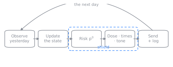
The daily loop. Yesterday’s observation updates the state, from which a risk is derived, then a dose, times and a tone. The whole thing is drawn at random under the shield, and logged for learning.
A belief state, not two numbers
Where the previous model kept two scalars, $C$ and $D$, the new one keeps a six-dimensional latent state:
$$ X_t = (M_t, H_t, R_t, B_t, F_t, Q_t) $$each in $[0, 1]$:
- $M$, motivation, the propensity to train spontaneously;
- $H$, the strength of habit;
- $R$, receptivity to messages;
- $B$, the weariness caused by solicitations (burden);
- $F$, physiological fatigue;
- $Q$, the reliability of commitments made.
I don’t know any of these values directly. So I keep a distribution rather than a point estimate: a cloud of a thousand weighted hypotheses, each one a plausible state. It’s a belief state, represented by a particle filter. At start-up, these hypotheses begin from moderate priors (motivation 0.55, habit 0.45, receptivity 0.50, weariness 0.10, reliability 0.60) and from wide uncertainty.
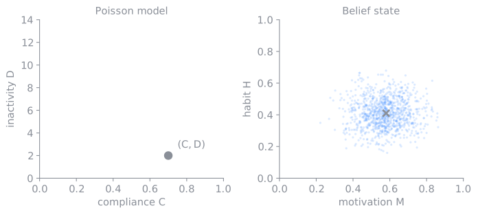
On the left, the Poisson model summarised the past in one point, (C, D). On the right, the belief state is a cloud of particles over motivation and habit: a distribution, and not a value.
At any moment, this cloud is summarised by the mean and spread of each dimension:
{
  "state": {
    "motivation":  {"mean": 0.58, "std": 0.11},
    "habit":       {"mean": 0.41, "std": 0.09},
    "receptivity": {"mean": 0.50, "std": 0.14},
    "weariness":   {"mean": 0.14, "std": 0.06},
    "fatigue":     {"mean": 0.05, "std": 0.04},
    "reliability": {"mean": 0.60, "std": 0.10}
  },
  "particles": 1000
}
Updating the state every day
This is the piece the Poisson model lacked. Every morning, before any decision, the coach corrects its estimate with what it observed the day before. The operation happens in two steps: first predict, then correct.
To predict is to take yesterday’s estimate and age it by one day. Motivation slides a little toward its mean, habit moves slowly, and the uncertainty widens: lacking new information, the coach is a little less sure of its state than it was yesterday. That is the role of a forgetting factor (discount 0.985 per day), which keeps an old observation from weighing forever.
To correct is to confront this prediction with what actually happened. The coach reconstructs the previous day’s action $A_{t-1}$ (the reminders sent, their times, their tone), then assembles an observation $O_t$ from the tracker and Garmin: did a session take place, at what load, did the person reply to the reminders, did they keep a planned slot. Every hypothesis of the state that fits this observation is reinforced, every hypothesis that contradicts it is weakened, and the cloud tightens.
These two steps are the two factors of a single Bayesian step, the prediction (the transition) and the correction (the likelihood):
$$ p(X_t \mid H_t) \;\propto\; \underbrace{p(O_t \mid X_t, A_{t-1})}_{\text{correction}} \cdot \underbrace{\int p(X_t \mid X_{t-1}, A_{t-1})\, p(X_{t-1} \mid H_{t-1})\, dX_{t-1}}_{\text{prediction}} $$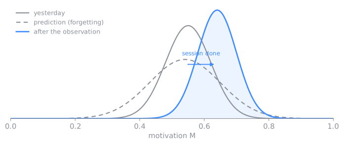
One estimation step, read on motivation. The prediction starts from yesterday’s state and widens (forgetting adds uncertainty). Observing a session recentres and tightens the cloud: that is the day’s posterior.
The likelihood of a session, the correction term, links the state and the action to the probability of having trained:
$$ \Pr(\text{sport}_t = 1 \mid X_t, A_t) = \sigma\big(\alpha_0 + M_t + H_t - F_t + \beta^{\top}\varphi(A_t)\big) $$where $\sigma$ is the logistic function, $\alpha_0 = -1.25$ a sceptical intercept, and $\varphi(A_t)$ a vector describing dose, times and tone. This equation carries the heart of the model, its separation into two terms:
- the spontaneous propensity, $M_t + H_t - F_t$, what the person would do alone;
- the intervention effect, $\beta^{\top}\varphi(A_t)$, what my reminders add to it.
An example makes the correction concrete. If the person trained yesterday with no reminder at all, the high-motivation hypotheses explain the observation better: the estimated motivation rises, and the day’s pressure drops. If they ignored three reminders without moving, the low-receptivity hypotheses are the ones that fit, and the coach will stay more discreet. The whole point is to attribute a session to the spontaneous propensity or to the effect of the reminders, and that is what justifies the last brick.
The risk of drift without intervention
Once the state is updated, the first question is simple: what would happen if I did nothing? I compute the spontaneous drift risk, the probability that no adequate session takes place within 24 to 48 hours if I cut all reminders:
$$ p^0_t = \Pr(\text{no session within 24-48 h} \mid do(A=0), H_t) = 1 - \mathbb{E}_{X}\big[\sigma(\alpha_0 + M + H - F)\big] $$The $do(A=0)$ is an intervention operator (do-calculus): it forces the absence of a reminder and cuts the estimated effect of messages, to isolate the person’s own behaviour. A high $p^0$ means “they may not move on their own”, so I should perhaps insist. A low $p^0$ means “they’ll train without me”, so I can stay discreet.
![A sigmoid of the probability of a session without a reminder against the spontaneous propensity, with the belief cloud, the expectation E[σ] and the risk p⁰ as the complement](/images/scop-drift-risk.svg)
The do(A=0) cuts the reminders: the probability of a session then follows σ(α₀ + M + H − F). Averaged over the belief cloud, it gives P(session | no reminder) = E[σ], and the drift risk is its complement, p⁰ = 1 - E[σ]. A high p⁰ calls for insisting, a low p⁰ for staying discreet.
Choosing the dose
The risk $p^0$ guides the number of reminders, but it doesn’t set it alone. For each dose $n \in \{0, \dots, 6\}$, I evaluate a utility that balances a benefit against several costs:
$$ U_t(n) = \underbrace{\alpha_b\, p^0_t\,(1 - e^{-\gamma_b n})}_{\text{benefit}} \;-\; \lambda_1 n \;-\; \lambda_2 n^2 \;-\; \lambda_B\, \mathbb{E}[B_t]\, n \;-\; \lambda_V\, \mathrm{Var} $$The benefit saturates with the dose (the fourth reminder adds less than the first) and grows with the risk $p^0$ (insisting helps more when the person disengages). The costs are a linear cost per reminder ($\lambda_1 = 0.018$), a convex cost that makes high doses rare ($\lambda_2 = 0.006$), a cost proportional to the estimated weariness ($\lambda_B = 0.045$), and a variance penalty that makes the coach cautious under uncertainty ($\lambda_V = 0.08$).
The number of reminders is then drawn at random, and not taken at the maximum, by a softmax over these utilities:
$$ \Pr(n_t = n \mid H_t) \;\propto\; \mathbf{1}[n \in N_t]\,\exp\!\big(U_t(n)/T_N\big) $$The temperature $T_N = 0.05$ lets a little randomness through around the best dose. This randomness has a precise role: it makes the causal learning of the last brick possible.
To avoid silence when insistence is needed, an adaptive floor imposes a minimum dose according to the risk:
floor(p⁰) = 0   if  p⁰ < 0.55
floor(p⁰) = 1   if  0.55 ≤ p⁰ < 0.75
floor(p⁰) = 2   if  p⁰ ≥ 0.75
It’s the direct answer to the Poisson model’s most visible flaw, those days drawn with zero reminders while the person was waiting for a nudge. A decision is then logged in full:
{
  "p0": 0.62,
  "floor": 1,
  "utilities":  {"0": -0.01, "1": 0.11, "2": 0.08, "3": 0.02},
  "propensity": {"0": 0.00, "1": 0.61, "2": 0.30, "3": 0.07},
  "drawn_dose": 1,
  "times": ["07:12"],
  "tone": ["encouraging"]
}
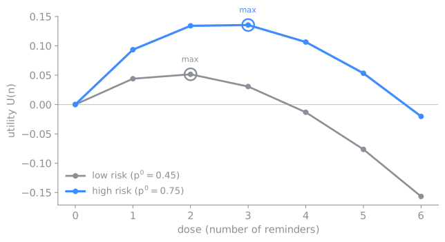
The utility of each dose, for a low risk and a high risk. The benefit saturates and the costs rise: the utility peaks around one dose, higher when the risk is higher.
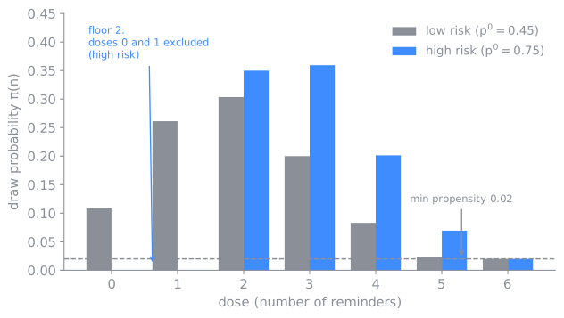
The dose is drawn at random rather than taken at the maximum: a tempered softmax picks it around the best utilities. The floor rules out low doses when the risk demands it, and the minimum propensity of 0.02 keeps every admissible dose reachable, which is what makes causal learning possible.
The shield
All this machinery is random, so it needs hard guardrails. The shield reduces the set of admissible doses before the draw. On some days, it reduces it to $\{0\}$: Sunday, in case of manifest overload, on suspicion of injury, or on the day of a return after a long stop (at least fourteen days without a session). In the first weeks, it caps the dose to ramp up gently.
The shield steps in a second time, just before sending. If the person has already done their session between the morning’s planning and the reminder’s time, the planned message loses its meaning: the shield cancels it or converts it into congratulations. This re-check guarantees that the action actually sent matches the real state, which matters as much for the experience as for learning.
The times and the tone
Once the dose is known, the reminders still need to be placed in the day and given a tone.
The times come from a hard-core point process, which draws minutes in the active window while respecting a minimum spacing of thirty minutes. Each minute gets a weight combining the hour, the proximity of a planned slot, the person’s historical receptivity, and a penalty for intrusive hours. It’s more constrained than a Poisson, which would violate the spacing.
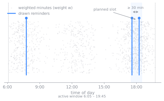
The weight of each minute combines the time of day, the proximity of a planned slot and receptivity. Reminders are drawn where the weight is high, at least thirty minutes apart (hard core).
The tone follows an ordinal scale, from the firmest to the warmest: hard, firm, neutral, encouraging, celebration. An ordinal logistic model picks one according to a latent score:
$$ z = \theta_0 + \theta_P\, p^0_t + \theta_M\,\text{misses}_t + \theta_i\, i - \theta_B B_t - \theta_F F_t + \theta_S\,\text{success}_t $$A high risk or missed commitments harden the tone; weariness, fatigue and recent successes soften it. A safety rule forbids the hard tone during a return or under overload, and the next reminder of the same day may rise one notch, without ever jumping abruptly.
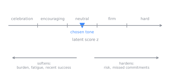
The tone is chosen on an ordinal scale, from the warmest to the sternest, according to the latent score z. Risk and missed commitments harden the tone; burden, fatigue and recent successes soften it.
Randomising to learn
This is the brick that truly sets this model apart from the previous one. Each decision (the dose, the times, the tone) is drawn at random with a known probability, which I log:
$$ \pi(A_t \mid H_t) = \pi_N(n_t \mid H_t)\cdot \pi_T(\tau_t \mid n_t, H_t)\cdot \pi_C(c_t \mid \tau_t, n_t, H_t) $$By randomising its own decisions and keeping the propensity score of each, the coach turns its history into a sequential randomised experiment, specific to a single person (N-of-1). As long as each reasonable dose keeps a non-zero probability (a positivity condition, set here to 0.02 at minimum), I can estimate the proper causal effect of dose, times and tone for this user.
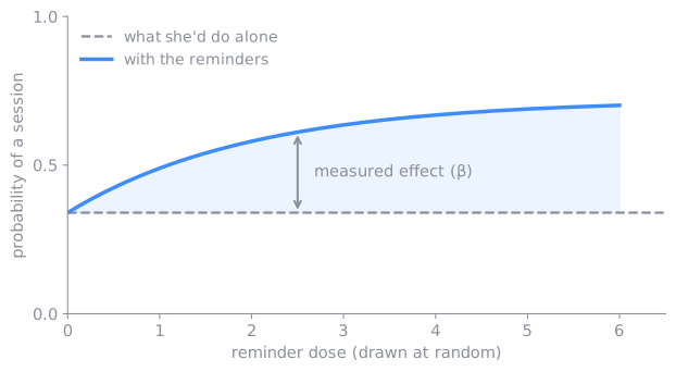
On days where the dose is drawn at random, the gap between what the person would do alone (the propensity) and what happens with the reminders gives the effect β. That gap is what randomisation lets us measure.
That is what the Poisson model couldn’t do. It scheduled without controlled randomisation, so it mixed spontaneous sport and the effect of reminders with no recourse. Here, if days with a high randomly drawn dose trigger more sessions, the model raises the estimated effect $\beta$; if the person trains without a reminder, it raises their motivation and reduces future pressure.
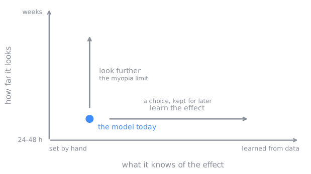
Learning the effect of the reminders and looking further ahead are two independent settings. The model learns little (parameters set by hand, by choice) and looks short (24-48 h, by design): two perpendicular directions, one a choice, the other the myopia limit.
Limits
This model fits the problem better than the Poisson process, but it remains a model, and a model always simplifies. Its most serious limits come from what it chooses to represent, and from what it leaves out.
The state is an abstraction. Six numbers and a few chosen equation shapes (a logistic likelihood, an additive propensity $M + H - F$, Gaussian noise) stand in for a person.
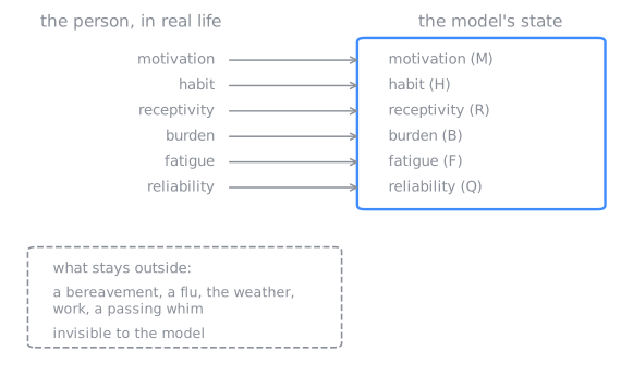
The model sums the person up in six numbers. Whatever acts outside this structure, a bereavement, a flu, the weather, stays outside the model.
The optimised objective is a proxy, a stand-in goal. The model maximises a number, the utility: an estimated habit gain, minus the cost of the reminders. What truly matters, that the person keeps going over time and is better for it, isn’t measured, so it enters no equation. This is Goodhart’s law: once a measure becomes a target, it stops being a good measure. The model can serve its number to perfection while drifting from the real goal, for instance by piling on reminders that trigger a session today, but wear the person down enough to mute the notifications next month.
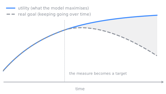
The utility the model maximises (the measure) can keep rising while the real goal, keeping going over time, declines. This is Goodhart’s drift.
The observation is too poor to decide. A person provides a few coarse signals a day: a session or not, a reply or not. Many different latent stories explain the same signals, so the belief over six dimensions stays loose, and at times confident when it shouldn’t be. The N-of-1 framing worsens the scarcity: each person is modelled alone, borrowing nothing from the behaviour of others.
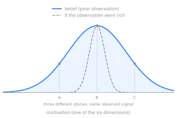
Three different latent stories (A, B, C) explain the same observed signal, so the belief stays wide. Dashed, the narrowness a rich observation would allow.
The decision is myopic. Each day, the model picks the dose that maximises the utility of the next 24 to 48 hours, and nothing beyond. It is a deliberate greedy policy: it weighs the present alone, never the weeks to come, where habit is actually built. Staying silent today to preserve receptivity for a nudge next week is beyond it by design. The term POMDP names the problem that the reminders pose, not the way this model settles it.
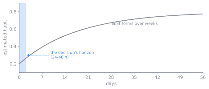
The decision optimises a 24-to-48-hour window (blue band), whereas habit forms over weeks (curve). The model is called a POMDP, but it does not plan over that long horizon.
Finally, experimentation has a price. To isolate the proper effect of a reminder, the model has to vary its decisions at random, and so to accept acting at times worse than its best estimate. On a single person, that price is paid for real, with no crowd to dilute it.
Conclusion
The Poisson process answered “when”. This model answers “should I nudge, and at what dose”. It keeps an estimate of the person’s state, corrects it every day with what they do, weighs the benefit and cost of each reminder, and draws its decisions at random with a known probability.
This last point is what truly sets it apart from the previous one. The Poisson process simulated a flow of reminders to be observed; this model treats a reminder as a decision that is made, for a person whose state stays hidden. By randomising its own decisions and keeping their propensity, it gives itself the means to estimate their causal effect for that person. It decides today, and it is built to learn from what it decides.